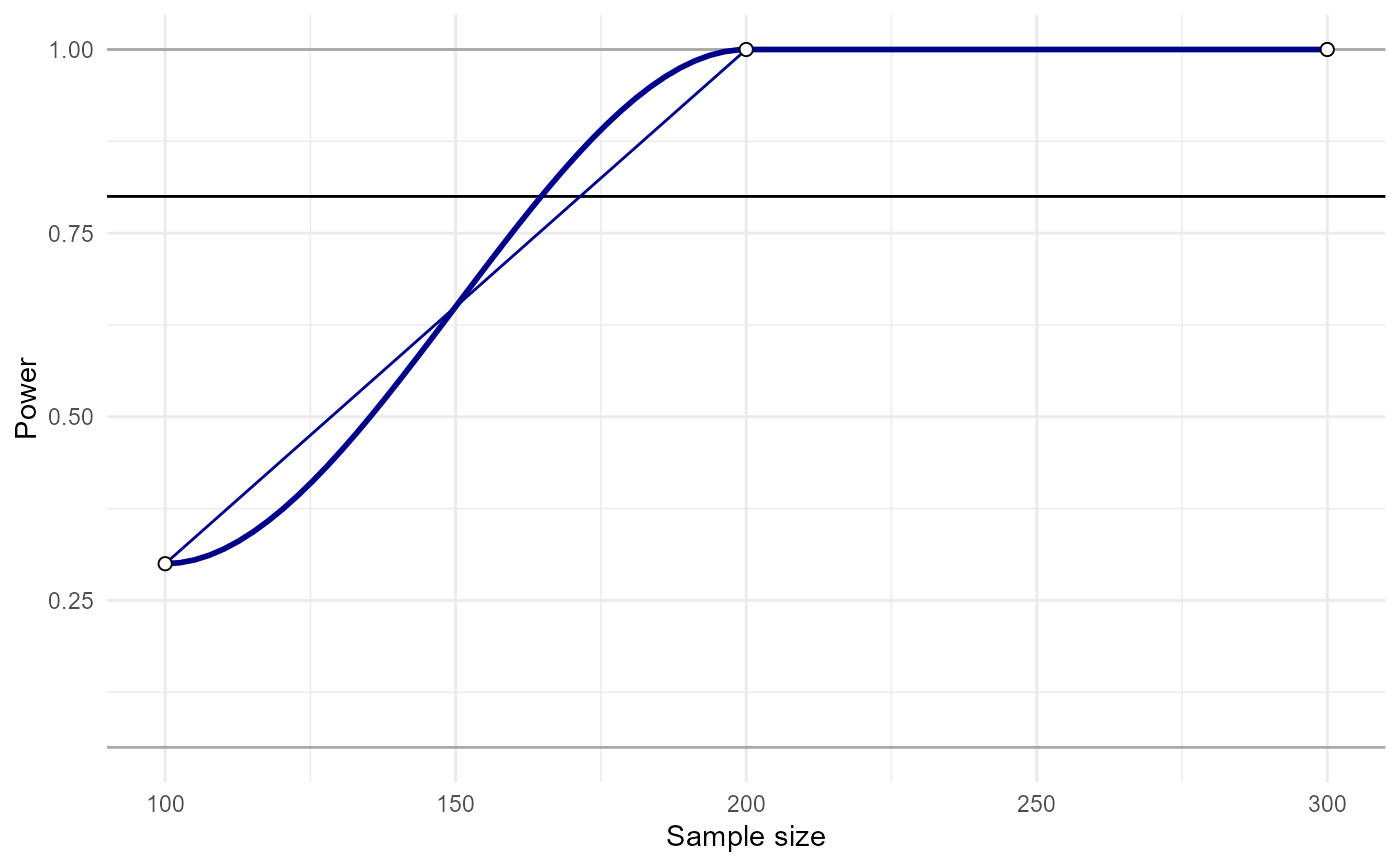
Plot power curve — plot_power_curve • InteractionPoweR

Plot the output of power_interaction().

Usage

plot_power_curve(
  power_data,
  x = NULL,
  group = NULL,
  facets = NULL,
  power_target = 0.8
)

Arguments

power_data: Data frame of results from power_interaction(). Can accept the raw results if up to 3 parameters were varied during simulation. Any more and data should be filtered first.
x: Optional, the x-axis of the plot. Default is the first variable after 'pwr'.
group: Optional, grouping variable for the line color. Default is the second variable after 'pwr', if present.
facets: Optional, grouping variable for plot facets. Default is the third variable after 'pwr' if present.
power_target: The target power. Default is 80%.

Value

A ggplot2 object

Examples

 power_analysis <- power_interaction(n.iter = 10,N = seq(100,300,by=100),
 r.x1.y = 0,r.x2.y = .1,r.x1x2.y = -.2,r.x1.x2 = .3,detailed_results = TRUE)
#> Performing 30 simulations
#> 
#> Attaching package: 'MASS'
#> The following object is masked from 'package:dplyr':
#> 
#>     select
 plot_power_curve(power_analysis)
#> Warning: span too small.   fewer data values than degrees of freedom.
#> Warning: pseudoinverse used at 99
#> Warning: neighborhood radius 101
#> Warning: reciprocal condition number  0
#> Warning: There are other near singularities as well. 10201
#> Warning: span too small.   fewer data values than degrees of freedom.
#> Warning: pseudoinverse used at 99
#> Warning: neighborhood radius 101
#> Warning: reciprocal condition number  0
#> Warning: There are other near singularities as well. 10201
#> Warning: no non-missing arguments to max; returning -Inf